Projectile Motion Initial Velocity: X and Y Made Easy!
Ever found yourself staring at a physics problem, knowing a projectile’s range and maximum height, but feeling completely stuck on how to calculate its launch speed? You’re not alone. The challenge of working backward to find the initial velocity is a common hurdle in understanding projectile motion. But this single value is the master key—it dictates the entire trajectory of an object in flight.
This guide is here to make it easy. We will demystify the process by breaking down initial velocity into its fundamental X and Y components. Forget the confusion; prepare for a clear, step-by-step journey through core kinematic equations and Trigonometry that will empower you to solve these problems with confidence and precision.
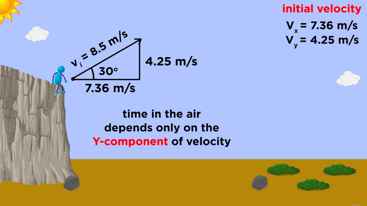
Image taken from the YouTube channel Professor Dave Explains , from the video titled Kinematics Part 3: Projectile Motion .
Navigating the physics of motion can often feel like a complex journey, but by understanding its fundamental elements, we can demystify even the most intricate scenarios.
The Launch Point: Unraveling Initial Velocity’s Secrets in Projectile Motion
Calculating the path of an object launched into the air – known as projectile motion – is a cornerstone of physics, crucial for everything from sports analytics to space exploration. However, one of the most common hurdles students and enthusiasts encounter is accurately determining the initial velocity of a projectile, especially when it’s launched at an angle. This initial push dictates everything that follows, yet its decomposition into usable components often presents a significant challenge.
Why Initial Velocity is the Key to Prediction
Understanding initial velocity isn’t merely an academic exercise; it’s the lynchpin for predicting the entire journey of a projectile. Without a precise grasp of this starting condition, accurately forecasting the object’s flight path becomes nearly impossible.
- Trajectory: The curved path a projectile follows is entirely shaped by its initial speed and direction. A slight alteration in initial velocity can dramatically change where an object lands or how high it reaches.
- Range (Horizontal Displacement): This refers to the total horizontal distance a projectile travels from its launch point to where it lands. Initial velocity directly influences how far an object will fly before gravity brings it back down.
- Maximum Height: The highest vertical point a projectile reaches during its flight is also a direct consequence of its initial upward velocity component. This is vital in fields requiring objects to clear obstacles or to understand the forces involved in a launch.
Our Mission: Simplifying Initial Velocity’s Complexity
The goal of this guide is to transform the daunting task of calculating initial velocity into a clear, manageable process. We’ll achieve this by breaking down the complex, single initial velocity vector into its more approachable, independent parts: the X and Y Components. By dissecting initial velocity into its horizontal (X) and vertical (Y) influences, we can analyze each dimension separately, significantly simplifying the problem. This approach adheres to the principle that horizontal and vertical motions in projectile problems are independent, governed by different forces (or lack thereof, in the case of horizontal motion ignoring air resistance).
What’s Ahead: Your Roadmap to Mastery
Prepare for a comprehensive, step-by-step journey designed to make the calculation of initial velocity feel "made easy." We will systematically explore the underlying principles, starting with the bedrock kinematic equations that describe motion, and then incorporating Trigonometry to effectively resolve initial velocity into its X and Y components. This guide will be punctuated with practical examples, demonstrating how to apply these concepts in real-world scenarios, ensuring you not only understand the theory but can confidently apply it.
Our exploration begins by uncovering the fundamental tools that allow us to break down complex motion: the power of vectors and the essential technique of deconstructing initial velocity into its X and Y components.
As we’ve begun to unlock the foundational concept of initial velocity in projectile motion, it’s crucial to delve deeper into its inherent nature and how we can break it down to simplify complex analyses.
Unlocking the Code: How Vectors Transform Initial Velocity
To truly master projectile motion, we must first understand the fundamental character of initial velocity itself. It’s not merely a speed; it’s a vector, carrying far more information than a simple number.
Initial Velocity: More Than Just Speed
In physics, initial velocity is defined as a vector quantity. This means it possesses two critical attributes:
- Magnitude: This is the "how fast" – the initial speed at which the object is launched.
- Direction: This is the "where to" – specifically, the angle of projection relative to a reference axis, typically the horizontal.
Consider a cannonball fired from the ground. Its initial speed tells us how powerful the launch was, but the angle at which the cannon is tilted tells us where it’s aimed. Both are indispensable for predicting its flight path.
Deconstructing the Vector: X and Y Components
The brilliance of vector analysis in projectile motion lies in its ability to simplify a single, angled motion into two much more manageable, independent movements. Any initial velocity vector can be conceptually resolved, or broken down, into two perpendicular and independent parts:
- Horizontal Velocity (vx): This component describes how fast the object is moving purely sideways.
- Vertical Velocity (vy): This component describes how fast the object is moving purely upwards or downwards at the moment of launch.
These two components act as the building blocks for understanding the entire trajectory. They are independent; what happens horizontally does not directly affect what happens vertically, and vice versa, except that they both operate over the same time duration.
The Critical Role of Trigonometry
When the angle of projection is involved, Trigonometry becomes an indispensable tool for resolving the initial velocity vector. Specifically, the sine and cosine functions allow us to calculate the magnitudes of the horizontal and vertical components from the initial speed and the launch angle.
Imagine a right-angled triangle where the hypotenuse is the initial velocity vector, and the two legs are its horizontal and vertical components. The angle of projection is one of the acute angles of this triangle.
Calculating the Components
Given the initial speed (let’s denote it as v
_initial) and the angle of projection (θ, measured from the horizontal), the formulas for calculating the horizontal velocity (vx) and the vertical velocity (vy) are:
- Horizontal Velocity (vx):
vx = v_initial**cos(angle)
- Vertical Velocity (vy):
vy = v_initial** sin(angle)
The following table summarizes these crucial relationships:
| Component | Formula | Description |
|---|---|---|
| Horizontal Velocity (vx) | v_initial
|
The portion of the initial velocity directed purely along the horizontal (X-axis). |
| Vertical Velocity (vy) | v
|
The portion of the initial velocity directed purely along the vertical (Y-axis), upward if angle > 0. |
Where:
v_initialis the magnitude of the initial velocity (the initial speed).θ(theta) is the angle of projection, measured from the horizontal.
The Power of Independence
One of the most profound concepts in projectile motion analysis is the conceptual independence of these X and Y Components. By breaking the initial velocity into vx and vy, we can analyze the horizontal motion separately from the vertical motion. This independence simplifies the problem greatly, allowing us to apply distinct sets of kinematic equations to each dimension without interference from the other. The only common link between these two independent motions is the time the projectile spends in the air.
Understanding how to deconstruct initial velocity into its independent horizontal and vertical components is the first secret to mastering projectile motion, and it sets the stage for analyzing each component’s behavior throughout the flight. Next, we will delve into the remarkable consistency of the horizontal velocity component.
Having successfully deconstructed the initial velocity into its independent X and Y components, we can now unveil the first crucial secret of projectile motion: the predictable and unwavering behavior of its horizontal dimension.
Gravity’s Blind Spot: The Unchanging Secret of Horizontal Motion
In the fascinating world of projectile motion, while objects trace graceful arcs through the air, one aspect remains remarkably consistent: their horizontal movement. This steadfastness is fundamental to understanding how far an object will travel.
The Unyielding Truth of Constant Horizontal Velocity (vₓ)
Imagine throwing a ball or firing a cannon. Once the object leaves its initial point, assuming we’re operating in an ideal scenario without air resistance, its horizontal velocity (vₓ) remains absolutely constant from launch to landing. This means if an object starts moving horizontally at 10 meters per second, it will continue to move horizontally at precisely 10 meters per second at every single point in its flight path. There are no forces acting horizontally to speed it up or slow it down.
Why Gravity Ignores the X-Component
The key to understanding this constancy lies in the nature of acceleration due to gravity (g). Gravity is a purely vertical force, always pulling objects straight downwards towards the Earth’s center. It has no horizontal component whatsoever.
Consider these points:
- Direction of Force: Gravity acts exclusively along the Y-axis (vertically).
- Lack of Horizontal Forces: In our idealized model, there are no forces pushing or pulling the projectile sideways (like wind or engine thrust).
- Newton’s First Law: An object in motion stays in motion with the same speed and in the same direction unless acted upon by an unbalanced force. Since no horizontal force acts on the projectile, its horizontal velocity remains unchanged.
Therefore, the powerful influence of gravity, which dramatically affects the vertical motion of a projectile, exerts zero impact on its horizontal motion.
The Simplified Kinematic Equation for Horizontal Motion
Because horizontal velocity (vₓ) is constant, the kinematic equations simplify significantly for the X-component. There’s no acceleration term to consider. The only equation we need relates horizontal displacement, horizontal velocity, and time:
Horizontal Displacement (x) = vx
**time
This equation is remarkably straightforward and powerful.
- x: Represents the horizontal displacement or range of the projectile (how far it travels horizontally).
- vₓ: Is the constant horizontal velocity.
- time: Refers to the total time of flight (the duration the object is in the air).
This equation highlights a direct relationship: the further something travels horizontally, the longer it must be in the air, or the faster its horizontal speed must be.
Determining Horizontal Velocity (vₓ)
You can find the horizontal velocity using different initial pieces of information:
-
If the Range (Horizontal Displacement) and Time of Flight are Known:
If you know how far the object traveled horizontally (xor Range) and how long it took to do so (timeor Time of Flight), you can easily rearrange the equation:
vx = Horizontal Displacement / Time of Flight
Example: If a projectile travels 100 meters horizontally in 5 seconds, its horizontal velocityvxis100 m / 5 s = 20 m/s. -
If the Initial Speed and Angle of Projection are Given:
As we established in the previous section, the initial velocity is a vector that can be broken into its X and Y components. If you know the initial speed (VinitialorV₀) and the angle at which it was launched (θ) relative to the horizontal, you can calculatevxusing trigonometry:
vx = Vinitial** cos(θ)
Example: If a projectile is launched at an initial speed of 30 m/s at an angle of 30 degrees above the horizontal, its horizontal velocityvxis30 m/s cos(30°) ≈ 30 m/s 0.866 = 25.98 m/s.
Key Horizontal Kinematic Equations
The table below summarizes the core equations governing horizontal motion in projectile problems, emphasizing their simplicity due to the absence of horizontal acceleration.
| Equation | Description | When to Use |
|---|---|---|
x = vx
|
Calculates horizontal displacement (range) given constant horizontal velocity and time. | To find how far an object travels horizontally or its range. |
vx = x / t |
Calculates constant horizontal velocity given horizontal displacement and time. | To determine the horizontal speed if range and time are known. |
vx = V_initial** cos(θ) |
Calculates initial horizontal velocity from the total initial speed and launch angle. | To find the horizontal component of velocity at the start of the motion. |
ax = 0 |
States that horizontal acceleration is zero (in ideal conditions). | A fundamental principle to remember for all horizontal projectile calculations. |
Understanding these unchanging truths of horizontal motion is crucial for predicting a projectile’s range. However, this is only half the story; the vertical journey, subject to the relentless pull of gravity, tells a far more dynamic tale.
While horizontal velocity offers a steady, unchanging pace, the vertical component of motion presents a far more dynamic and captivating story.
The Relentless Pull: Understanding Vertical Velocity’s Dance with Gravity
Unlike its horizontal counterpart, vertical velocity (vy) is in a constant state of flux, continuously changing throughout a projectile’s flight. This relentless alteration is solely due to the ever-present, downward force of acceleration due to gravity (g). Understanding this dynamic interplay is crucial for accurately predicting and analyzing projectile trajectories.
Gravity’s Unyielding Influence
The heart of vertical motion’s variability lies with acceleration due to gravity (g). This constant acceleration pulls all objects downwards, causing their vertical velocity to decrease as they ascend and increase as they descend.
- Definition:
gis approximately -9.8 m/s² in the metric system or -32 ft/s² in the imperial system. - Direction: The negative sign signifies that
galways acts downward, opposing upward motion and enhancing downward motion. Whether an object is moving up or down, gravity consistently attempts to pull it towards the Earth’s center.
The Kinematic Toolkit for Vertical Motion
To precisely quantify these changes in vertical velocity, we employ a set of fundamental kinematic equations. These equations relate initial vertical velocity, final vertical velocity, vertical displacement, time, and the constant acceleration due to gravity. They are the essential tools for dissecting the vertical journey of any projectile.
Here are the key variables and equations:
vy0: Initial vertical velocityvyf: Final vertical velocityΔy: Vertical displacement (change in vertical position)t: Time intervalg: Acceleration due to gravity (always negative for downward acceleration)
| Equation | Description |
|---|---|
vyf = vy0 + g
|
Relates final vertical velocity to initial vertical velocity, acceleration due to gravity, and time. Useful when time is known or sought, and displacement is not explicitly involved. |
Δy = vy0** t + 0.5 g t² |
Calculates vertical displacement based on initial vertical velocity, time, and acceleration due to gravity. Useful when final vertical velocity is not explicitly involved. |
vyf² = vy0² + 2 g Δy |
Connects final and initial vertical velocities with vertical displacement and acceleration due to gravity. Useful when time is not known or sought. |
Δy = ((vy0 + vyf) / 2)
|
Relates vertical displacement to the average vertical velocity and time. Useful when acceleration is constant, and g is implicitly accounted for by vy0 and vyf. |
Key Moments in a Projectile’s Vertical Journey
Certain points in projectile motion offer unique insights into vertical velocity:
-
At the Maximum Height: This is a critical juncture. As an object travels upward, its vertical velocity steadily decreases due to gravity. Precisely at the maximum height, the object momentarily stops moving upward before beginning its descent. At this exact instant, its vertical velocity (vy) becomes zero. This fact is incredibly useful for solving problems, as
vyf = 0at the peak of the trajectory. -
Symmetry of Vertical Velocity: For any projectile launched from and returning to the same horizontal level (e.g., ground level), there’s a beautiful symmetry to its vertical motion. At equivalent heights during both ascent and descent, the magnitude of the vertical velocity will be the same, but its direction will be opposite. For example, if an object has an upward vertical velocity of +5 m/s at a certain height on its way up, it will have a downward vertical velocity of -5 m/s at the same height on its way down.
Unlocking Initial Vertical Velocity
The kinematic equations, combined with the understanding of these key moments, allow us to determine the initial vertical velocity (vy0) if other parameters are known:
-
Using Maximum Height: If you know the maximum height (
Δy) reached, you can use the fact thatvyf = 0at that peak. The equationvyf² = vy0² + 2** g Δybecomes0 = vy0² + 2 g**Δy, which can be rearranged to solve for
vy0. -
Using Time of Flight: If you know the total time of flight (
t) for a symmetrical trajectory (starting and ending at the same height), the time to reach the maximum height is half the total time (t/2). You can then usevyf = vy0 + g** twithvyf = 0andt_peak = t/2to findvy0. Alternatively, if the starting and ending heights differ, you can useΔy = vy0 t + 0.5 g * t²directly ifΔyandtare known.
By mastering these principles and the application of the kinematic equations, you gain a powerful lens through which to analyze the intricate vertical dynamics of any object in flight. Now that we understand the independent behaviors of horizontal and vertical velocities, it’s time to learn how to combine them back into a unified initial velocity.
Having meticulously navigated the intricacies of how vertical velocity changes throughout a projectile’s flight, we now hold two crucial pieces of the puzzle: the initial horizontal velocity (vx) and the initial vertical velocity (vy). But these are merely components; the true launch requires their harmonious combination.
From Pieces to Power: Assembling the Full Picture of Initial Velocity
Imagine vx and vy as the blueprints for a grand construction – you have the length and the height, but to understand the full structure, you need to see how they fit together to form the diagonal, the true path of ascent. This section reveals how we reconstruct the complete initial velocity of a projectile, not just as isolated components, but as a single, powerful vector with both magnitude and direction.
The Vector Blueprint: Combining Horizontal and Vertical Components
When a projectile is launched, its initial velocity isn’t simply a number; it’s a vector, meaning it has both a speed (magnitude) and a direction (angle). We’ve previously isolated this vector into two perpendicular components:
- Horizontal Velocity (
vx): This component remains constant (assuming no air resistance) and dictates how far the projectile travels horizontally. - Vertical Velocity (
vy): This component changes due to gravity but represents the initial upward or downward thrust.
These two components act independently but simultaneously, creating a right-angled triangle where vx and vy are the two perpendicular sides. The hypotenuse of this triangle represents the overall initial velocity vector (v
_initial).
Unveiling the Magnitude: The Power of the Pythagorean Theorem
To find the magnitude (the speed) of the overall initial velocity (v_initial), we can leverage a fundamental geometric principle: the Pythagorean Theorem. Just as you’d find the length of the hypotenuse of a right-angled triangle given its two sides, you can find v
_initial given vx and vy.
The formula is expressed as:
v_initial = sqrt(vx^2 + vy^2)
Where:
vis the magnitude of the initial velocity._initial
vxis the initial horizontal velocity component.vyis the initial vertical velocity component.
This equation tells us that the square of the initial velocity’s magnitude is equal to the sum of the squares of its horizontal and vertical components. By taking the square root, we get the actual speed at which the projectile was launched.
Pinpointing the Direction: Calculating the Angle of Projection
Knowing the speed is only half the story; we also need to know the initial direction, commonly referred to as the angle of projection (theta). This angle is typically measured with respect to the horizontal. Since vx, vy, and v_initial form a right-angled triangle, we can use basic Trigonometry to determine this angle.
Specifically, the tangent of the angle of projection (theta) is the ratio of the opposite side (vy) to the adjacent side (vx). To find the angle itself, we use the inverse tangent function (also known as arctan or tan^-1):
theta = arctan(vy / vx)
Where:
thetais the angle of projection (in degrees or radians, depending on your calculator settings).vyis the initial vertical velocity component.vxis the initial horizontal velocity component.
This angle is crucial for understanding the trajectory. A larger theta means a steeper, higher trajectory, while a smaller theta results in a flatter, longer trajectory (for the same initial speed).
Putting it All Together: Step-by-Step Examples
Let’s walk through a couple of common problem scenarios to see how vx and vy (derived from other given information) are combined to find the overall initial velocity and its angle.
Example 1: Given Time of Flight and Horizontal Range
Problem: A projectile is launched from the ground and lands at the same height. Its total time of flight is 4 seconds, and its horizontal range is 80 meters. Calculate its initial velocity (magnitude and angle). (Assume g = 9.8 m/s^2).
Solution:
-
Determine
vx:- Horizontal velocity is constant:
vx = Range / Time of Flight vx = 80 m / 4 s = 20 m/s
- Horizontal velocity is constant:
-
Determine
vy(initial vertical velocity for a symmetric trajectory):- For a symmetric flight, the time to reach maximum height is half the total time of flight:
t._up = T / 2 = 4 s / 2 = 2 s
- At maximum height, the final vertical velocity is 0. Using
v_f = vi + atup: 0 = vy + (-g)**t
_up
vy = g** t_up = 9.8 m/s^2**2 s = 19.6 m/s
- For a symmetric flight, the time to reach maximum height is half the total time of flight:
-
Calculate
v_initial magnitude:
v_initial = sqrt(vx^2 + vy^2)v_initial = sqrt((20 m/s)^2 + (19.6 m/s)^2)
v_initial = sqrt(400 + 384.16)v(approx.)_initial = sqrt(784.16) = 28.00 m/s
-
Calculate
theta(angle of projection):theta = arctan(vy / vx)theta = arctan(19.6 / 20)theta = arctan(0.98) = 44.4°(approx.)
Result: The projectile was launched with an initial velocity of approximately 28.00 m/s at an angle of 44.4° above the horizontal.
Example 2: Given Horizontal Range and Maximum Height
Problem: A projectile launched from the ground reaches a maximum height of 10 meters and has a horizontal range of 60 meters. Determine its initial velocity (magnitude and angle). (Assume g = 9.8 m/s^2).
Solution:
-
Determine
vy(initial vertical velocity):- At maximum height,
v_fy = 0. Usingvfy^2 = viy^2 + 2ady: 0^2 = vy^2 + 2** (-g)**h
_max
vy^2 = 2** g**h_max
vy = sqrt(2** 9.8 m/s^2**10 m)
vy = sqrt(196) = 14 m/s
- At maximum height,
-
Determine time to maximum height (
t_up):
- Using
v_fy = viy + atup: 0 = 14 m/s + (-9.8 m/s^2)** t_up
t_up = 14 / 9.8 = 1.43 s(approx.)
- Using
-
Determine total time of flight (
T):- For a symmetric trajectory,
T = 2 t(approx.)_up = 2
1.43 s = 2.86 s
- For a symmetric trajectory,
-
Determine
vx:- Horizontal velocity is constant:
vx = Range / T vx = 60 m / 2.86 s = 20.98 m/s(approx.)
- Horizontal velocity is constant:
-
Calculate
v_initialmagnitude:v_initial = sqrt(vx^2 + vy^2)
v_initial = sqrt((20.98 m/s)^2 + (14 m/s)^2)v_initial = sqrt(439.96 + 196)
v_initial = sqrt(635.96) = 25.22 m/s(approx.)
-
Calculate
theta(angle of projection):theta = arctan(vy / vx)theta = arctan(14 / 20.98)theta = arctan(0.667) = 33.7°(approx.)
Result: The projectile was launched with an initial velocity of approximately 25.22 m/s at an angle of 33.7° above the horizontal.
Summary Table: Navigating Problem Types
This table summarizes how initial velocity components are found from common problem scenarios, leading to the calculation of the overall initial velocity’s magnitude and angle.
| Problem Type (Given…) | How vx is Determined (Pre-calculation) |
How vy is Determined (Pre-calculation) |
vinitial Magnitude Formula (vi) |
theta Angle Formula (θ) |
|---|---|---|---|---|
Direct vx & vy Provided |
Given directly | Given directly | sqrt(vx^2 + vy^2) |
arctan(vy / vx) |
| Range (R) & Time of Flight (T) | R / T |
(g
(for symmetric flight) |
sqrt((R/T)^2 + ((g**T)/2)^2) |
arctan(((g
|
| Range (R) & Max Height (h
_max) |
First calculate T = 2** sqrt(2
, then R / T |
sqrt(2** g
(for symmetric flight) |
sqrt((R/T)^2 + (sqrt(2**g
|
arctan(sqrt(2**g
|
Initial Velocity (v_i) & Angle (θ) (Working backwards) |
v
|
v_i * sin(θ) |
(Already known) | (Already known) |
By skillfully combining the horizontal and vertical components, we gain a complete understanding of the projectile’s launch conditions, a fundamental step before we dive into how these principles translate into real-world scenarios and common pitfalls.
Having successfully pieced together the horizontal and vertical components to reveal the full picture of initial velocity, it’s time to put this powerful understanding to practical use and steer clear of common missteps that can derail your calculations.
Beyond the Blueprint: Launching Success and Evading Projectile Motion’s Hidden Traps
Understanding projectile motion isn’t just an academic exercise; it’s a fundamental concept with far-reaching implications across various fields. From the precise trajectory of a golf ball to the launch sequence of a rocket, calculating initial velocity accurately is paramount. However, the path to mastery is often riddled with common errors that can lead to incorrect results. This section delves into real-world applications, highlights typical pitfalls, and equips you with essential problem-solving strategies to ensure your calculations are consistently accurate.
Real-World Trajectories: Where Initial Velocity Matters
The ability to calculate initial velocity from its components transforms theoretical physics into a powerful tool for analyzing and predicting movement in our world.
Sports Analytics: Precision in Play
- Golf: Professional golfers and coaches use sophisticated motion capture systems to analyze the initial velocity of the club head and the ball immediately after impact. This data helps optimize swing mechanics, club face angle, and loft to achieve specific launch angles and distances, directly impacting performance.
- Baseball: Pitchers’ initial release velocity and angle are crucial. Analysts use these figures to predict ball trajectory, helping hitters anticipate pitches. Similarly, the initial velocity of a batted ball determines if it’s a pop-up, a line drive, or a home run, offering insights into player performance and equipment design.
Engineering Marvels: Guiding the Unseen
- Rocket Launches: In aerospace engineering, precisely calculating the initial velocity and launch angle is critical for rockets and satellites to escape Earth’s gravity and achieve their intended orbits. Every kilogram of fuel, every degree of launch angle, and every meter per second of initial velocity is meticulously planned.
- Ballistic Trajectories: From military applications to forensic science, understanding the initial velocity of a projectile (like a bullet) is vital for determining its range, impact point, and even the origin of a shot. This requires careful application of kinematic equations.
Everyday Physics: Unveiling the Obvious
Even in simpler scenarios, the principles apply. Thinking about the initial velocity helps in tasks like:
- Aiming a garden hose to water plants at a specific distance.
- Throwing a ball to land exactly in a friend’s hands.
- Designing water features in a park for a desired spray height and distance.
Navigating the Labyrinth: Common Projectile Motion Pitfalls
While the concepts of projectile motion might seem straightforward, several common mistakes can lead to incorrect answers. Recognizing these traps is the first step toward avoiding them.
| Common Pitfall in Projectile Motion | Strategy to Avoid It |
|---|---|
| Confusing X and Y Components | Always analyze horizontal (X) and vertical (Y) motions completely separately. Remember, horizontal velocity is constant (if air resistance is ignored), while vertical velocity changes due to gravity. |
| Incorrect Sign for Acceleration Due to Gravity (g) | Consistently define your positive and negative directions. If ‘up’ is positive, then ‘g’ (which acts downwards) should be -9.8 m/s². If ‘down’ is positive, ‘g’ is +9.8 m/s². Stick to one convention throughout the problem. |
| Misapplying Kinematic Equations | Ensure you’re using the correct kinematic equation for the variable you’re trying to find and that all other variables in the equation are known for the same component (X or Y) and same time interval. |
| Overlooking the Angle of Projection | Always break the initial velocity vector into its X (V₀x = V₀ cosθ) and Y (V₀y = V₀ sinθ) components immediately. Failing to do so prevents correct application of kinematic equations to each dimension. |
| Mixing Up Time (t) Between X and Y | Time is the only variable common to both the horizontal and vertical components of projectile motion. It’s often the bridge between the two dimensions. Don’t use different ‘t’ values for X and Y for the same flight duration. |
Your Toolkit for Success: Essential Problem-Solving Strategies
Approaching projectile motion problems systematically can significantly improve accuracy and understanding.
- Draw a Clear Diagram: Always start by sketching the scenario. Label the initial position, final position, initial velocity vector (V₀) with its angle (θ), and the direction of acceleration due to gravity. This visual aid clarifies the problem.
- List Knowns and Unknowns: Create two separate lists: one for the horizontal (X) components and one for the vertical (Y) components. Clearly identify what values are given and what you need to find.
- X-components: Vₓ, Δx, t
- Y-components: V₀y, Vy, Δy, a
_y (-g), t
- Choose Appropriate Kinematic Equations: Based on your knowns and unknowns for each component, select the relevant kinematic equations. Remember that horizontal motion typically only uses Δx = Vₓt (since Vₓ is constant), while vertical motion uses equations involving acceleration
a_y = -g. - Break Down the Problem: If the problem seems complex, break it into smaller, manageable parts. For instance, consider the motion to the peak of the trajectory, then the motion from the peak to the ground, or consider the entire flight time.
- Use Consistent Units: Ensure all your measurements are in a consistent system (e.g., meters, kilograms, seconds).
The Unseen Hand: Acknowledging Air Resistance
It’s important to briefly note that in most introductory physics problems, we simplify projectile motion by ignoring air resistance. In reality, air resistance (or drag) significantly impacts the trajectory of an object, especially at high speeds or for objects with large surface areas relative to their mass. It acts as a force opposing the object’s motion, reducing both its horizontal range and maximum height. While its effects are complex and generally not considered in basic calculations, being aware of its presence is crucial for understanding real-world scenarios.
By internalizing these practical applications and mastering the art of avoiding common pitfalls, you’re now poised to take complete command of your initial velocity calculations in any scenario.
Having explored practical applications and learned to sidestep common traps in projectile motion, our next step is to delve into the foundational element that dictates a projectile’s entire journey: its initial velocity.
Beyond the Launchpad: Deconstructing Initial Velocity for Projectile Mastery
At the heart of every successful projectile motion analysis lies a profound understanding of its initial velocity. This isn’t just a simple speed; it’s a vector quantity, possessing both magnitude and direction, which sets the entire trajectory into motion. Recognizing this fundamental nature allows us to apply a powerful simplification: breaking down this complex single vector into its more manageable horizontal (X) and vertical (Y) components. This decomposition is the cornerstone of simplifying seemingly intricate projectile problems, transforming them into a pair of more straightforward, independent analyses.
The Power of Component Decomposition
Imagine launching a ball. It doesn’t just go "forward" and "up" simultaneously as one indivisible action. Instead, its initial push can be thought of as two separate impulses: one purely horizontal and one purely vertical. This mental model is precisely what component decomposition enables.
- Horizontal Component (Vx): This component dictates how fast the projectile moves along the ground. Crucially, in the absence of air resistance, this velocity remains constant throughout the projectile’s flight. There are no forces acting horizontally to accelerate or decelerate it.
- Vertical Component (Vy): This component dictates how high the projectile will go and how long it will stay in the air. It is constantly affected by the force of gravity, causing the projectile to accelerate downwards (or decelerate as it moves upwards).
By separating the initial velocity vector into these orthogonal (perpendicular) components, we can analyze the horizontal and vertical motions independently. The X-motion becomes a simple constant velocity problem, while the Y-motion becomes a constant acceleration problem under gravity. This dramatically simplifies the application of kinematic equations, turning a complex 2D problem into two more digestible 1D problems.
Essential Tools: Vectors, Trigonometry, and Kinematics
To effectively break down initial velocity and then utilize those components, a solid grasp of specific mathematical and physical tools is paramount.
Understanding Vectors
A vector is a quantity that has both magnitude (size) and direction. Initial velocity is a prime example. When we represent it graphically, it’s an arrow whose length indicates the speed and whose orientation indicates the direction of launch. Understanding how to represent, add, and resolve vectors is the foundational skill for any projectile motion problem.
The Indispensable Role of Trigonometry
Trigonometry is the bridge that allows us to decompose an initial velocity vector into its X and Y components. Given the initial speed (magnitude) and the launch angle (direction relative to the horizontal), we use the basic trigonometric functions:
- Cosine (cos): Used to find the horizontal component (adjacent side)
Vx = V_initial
**cos(theta)
- Sine (sin): Used to find the vertical component (opposite side)
Vy = V_initial** sin(theta)
Where V_initial is the magnitude of the initial velocity and theta is the launch angle. A firm understanding of these relationships is non-negotiable for accurately setting up your problems.
Applying Kinematic Equations
Once the initial velocity is resolved into its components, we apply the appropriate kinematic equations (equations of motion) to each dimension:
- For Horizontal Motion (X-axis): Since
ax = 0(assuming no air resistance), we primarily use:Δx = Vx(displacement equals velocity times time)**t
- For Vertical Motion (Y-axis): Here,
ay = -g(acceleration due to gravity, approximately -9.8 m/s²). We use:Δy = Vy** t + 0.5 ay t^2Vfy = Vy + ay**t
Vfy^2 = Vy^2 + 2** ay * Δy
The crucial link between these two independent sets of equations is time (t), which is the same for both the horizontal and vertical journeys.
Sharpening Your Skills: Practice Makes Perfect
Like any skill, mastering initial velocity in projectile motion comes with consistent practice. Do not shy away from diverse scenarios; they are your training ground. Work through problems that involve:
- Launching from ground level to ground level.
- Launching from a height (e.g., cliff) to the ground.
- Targeting a specific horizontal or vertical distance.
- Calculating maximum height or time of flight.
- Finding the required launch angle for a given range.
Each problem type reinforces your understanding of component decomposition, the application of kinematic equations, and the strategic use of time as the unifying variable. The more you practice, the more intuitive these concepts become, building a robust problem-solving toolkit.
Your Path to Projectile Mastery
With these ‘secrets’—the strategic decomposition of initial velocity into X and Y components, the precise application of vectors and trigonometry, and the thoughtful deployment of kinematic equations—you are now equipped to tackle virtually any initial velocity problem in projectile motion with ease. This foundational understanding not only demystifies complex trajectories but empowers you with the analytical tools to predict and understand the path of any launched object.
Armed with this comprehensive understanding, you are now ready to not only solve but truly comprehend the dynamics of any projectile, laying the groundwork for even more advanced physics applications.
Frequently Asked Questions About Initial Velocity in Projectile Motion
What are the X and Y components of initial velocity?
The initial velocity of a projectile is broken down into two independent parts: a horizontal component (vx) and a vertical component (vy). This split simplifies problem-solving, as gravity only affects the vertical motion.
How do you find the initial velocity components from the launch speed and angle?
You can use basic trigonometry. The horizontal component (vx) is calculated as v * cos(θ), and the vertical component (vy) is v * sin(θ), where ‘v’ is the initial speed and ‘θ’ is the launch angle relative to the horizontal.
Why is separating velocity into X and Y components useful?
Separating velocity is the core of how do you calculate initial velocity projectile motion physics using x and y concepts. It allows you to analyze the constant horizontal motion and the vertically accelerated motion (due to gravity) independently, making complex problems much easier to solve.
Can you determine initial velocity from the projectile’s path?
Yes. If you know key information like the maximum height and the total horizontal distance (range), you can use kinematic equations. By working backward from these points, you can solve for the initial X and Y velocity components.
The secret to mastering projectile motion isn’t about memorizing complex formulas, but about strategic thinking. As we’ve seen, the most powerful approach is to deconstruct the seemingly complex initial velocity vector into its two simpler, manageable parts: the horizontal (X) and vertical (Y) components. This method transforms a daunting problem into a straightforward puzzle.
By consistently applying the principles of vectors, the rules of Trigonometry, and the appropriate kinematic equations for each axis, you now have a reliable framework for analysis. We encourage you to practice with diverse scenarios to build your confidence. With these ‘secrets’ unlocked, you are now fully equipped to tackle virtually any initial velocity problem with the analytical skill of an expert.
