Master Average Velocity on V-T Graphs: The Ultimate 3 Steps
Ever stared at a jumble of lines on a Velocity-Time Graph and felt like you were trying to read a secret code? You’re not alone. These graphs are the visual language of motion in physics, telling a dynamic story of an object’s journey—its speed, direction, and acceleration. But how do you boil down that entire story into a single, meaningful number?
The answer lies in mastering one crucial concept: Average Velocity. Forget the confusion. This guide is your key to unlocking that code. We will walk you through an ultimate, foolproof 3-step method to confidently calculate average velocity from any V-T graph, turning complex problems into straightforward solutions. Whether you’re a high school student gearing up for an exam or a college student solidifying your kinematics foundation, get ready to transform these graphs from a source of frustration into your favorite physics tool.
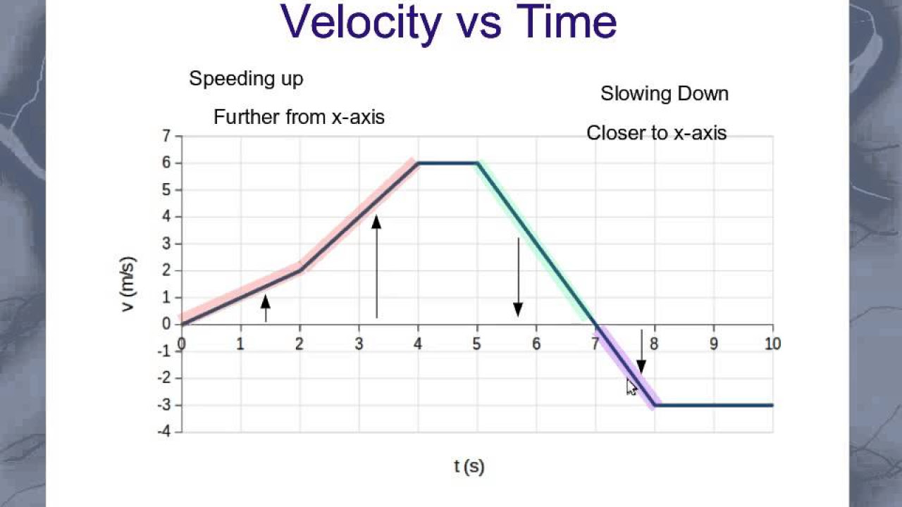
Image taken from the YouTube channel Jennifer Cash , from the video titled Interpreting Velocity graphs .
To truly grasp how objects move and change their speed, we must first understand the powerful tools that visualize such dynamic processes.
Your Roadmap to Motion: Conquering Velocity-Time Graphs and Average Velocity
Welcome to an essential guide designed to demystify one of the most fundamental concepts in physics: Velocity-Time Graphs. Whether you’re a high school student tackling kinematics for the first time or a college student seeking to solidify your understanding, this section will equip you with the knowledge to confidently interpret these graphs and, crucially, to master Average Velocity calculations. We’ll navigate the world of changing speeds and directions, transforming complex motion into clear, visual stories.
Why Velocity-Time Graphs are Indispensable in Physics
At their core, Velocity-Time Graphs are much more than just lines on a grid; they are powerful visualization tools that offer a complete picture of an object’s motion. These graphs plot an object’s velocity (speed with direction) on the vertical (y) axis against time on the horizontal (x) axis. By looking at the shape and slope of the line, physicists can instantly understand:
- Motion Visualization: Is the object moving forward or backward? Is it speeding up, slowing down, or moving at a constant velocity?
- Acceleration: The slope of a velocity-time graph directly represents the object’s acceleration. A steep slope indicates rapid acceleration, a gentle slope shows slow acceleration, and a horizontal line signifies zero acceleration (constant velocity).
- Displacement: As we’ll soon discover, the area between the line and the time axis reveals the object’s displacement.
Understanding these graphs is fundamental because they provide an intuitive and comprehensive way to analyze, predict, and describe the behavior of moving objects, making complex scenarios much easier to understand.
Decoding Average Velocity: More Than Just Speed
While instantaneous velocity tells you an object’s speed and direction at a precise moment, Average Velocity provides a broader perspective. It describes the overall change in an object’s position (displacement) over a specific Time Interval, regardless of the fluctuations in its speed during that period.
Why is this important? Imagine a car trip. You might speed up, slow down, stop at lights, and then accelerate again. Your speedometer shows your instantaneous velocity. However, to know how quickly you covered the entire distance from point A to point B, you’d calculate your average velocity. It smooths out all the transient changes, giving you a single value that characterizes the overall rate of motion. Calculating average velocity from a velocity-time graph involves understanding both the total displacement and the total time elapsed.
Your 3-Step Blueprint for Success
To empower you with the skills to confidently interpret these graphs and solve related problems, we’ve broken down the process into an ultimate 3-step approach. This blueprint is designed to build your understanding progressively, ensuring you grasp each concept before moving to the next. For all high school and college physics students, these steps will be your reliable guide:
- Unlocking Displacement: We’ll uncover how to calculate the total change in position from a velocity-time graph.
- Calculating Average Velocity: With displacement in hand, we’ll then learn the straightforward method for determining average velocity.
- Applying Your Knowledge: Finally, we’ll put everything together, working through examples that reinforce your understanding and problem-solving abilities.
Ready to embark on this journey? Let’s begin by tackling the first crucial step: understanding how the space under the curve reveals an object’s movement.
As we begin to navigate the fascinating world of velocity-time graphs, our first crucial stop is understanding how these visual representations reveal the true movement of an object.
Beyond the Lines: Unveiling Displacement Through the Area Under the Curve
When we talk about an object’s motion, we often hear terms like distance and speed. However, to truly understand how an object has changed its position and to calculate its average velocity, we need to focus on a more precise concept: displacement. Unlike total distance, which measures the entire path traveled, displacement measures the straight-line distance and direction from the starting point to the ending point. On a velocity-time graph, unlocking this crucial first step for calculating average velocity isn’t as complex as it might seem; it’s hidden in the visual space between the graph line and the time axis.
Defining Displacement: The Area Under the Curve
On a velocity-time graph, the displacement of an object over a chosen time interval is precisely represented by the Area Under the Curve. Imagine drawing a line straight down from the graph line to the time (x) axis, for every point within your chosen time frame. The space enclosed by the graph line, the time axis, and the vertical lines marking the start and end of your interval—that’s your displacement. This fundamental principle allows us to translate graphical information into a concrete measure of an object’s change in position.
Calculating Displacement for Common Shapes
To find the area under the curve, we often break down the graph into familiar geometric shapes. Depending on how an object’s velocity changes over time, these shapes will typically be rectangles, triangles, or trapezoids.
Rectangles: For Periods of Constant Velocity
When an object moves at a constant velocity, its line on the velocity-time graph will be horizontal. The area under this horizontal line, over a specific time interval, forms a perfect rectangle. Calculating its area is straightforward:
- Formula:
Displacement = Velocity × Time(which is simply thelength × widthof the rectangle). - Example: If an object travels at 5 m/s for 10 seconds, the displacement is 5 m/s × 10 s = 50 meters.
Triangles: For Periods of Constant Acceleration (Starting or Ending at Rest)
If an object undergoes constant acceleration (or deceleration) and starts from rest (velocity = 0) or comes to a complete stop, the shape formed under its graph line will be a triangle. This represents a steady increase or decrease in velocity.
- Formula:
Displacement = 0.5 × Base × Height - In V-T terms:
Displacement = 0.5 × Time Interval × Change in Velocity(where the ‘height’ is the maximum velocity reached or the initial velocity if decelerating to zero). - Example: An object accelerates steadily from 0 m/s to 10 m/s in 5 seconds. The displacement is 0.5 × 5 s × 10 m/s = 25 meters.
Trapezoids: For General Constant Acceleration
For more general cases of constant acceleration, where an object starts at one non-zero velocity and accelerates (or decelerates) to another non-zero velocity, the shape under the curve is a trapezoid. This is a common scenario in many real-world movements.
- Formula:
Displacement = 0.5 × (Sum of Parallel Sides) × Height - In V-T terms:
Displacement = 0.5 × (Initial Velocity + Final Velocity) × Time Interval(here, the parallel sides are the initial and final velocities, and the height is the time interval). - Example: An object starts at 2 m/s and accelerates to 8 m/s over 4 seconds. The displacement is 0.5 × (2 m/s + 8 m/s) × 4 s = 0.5 × 10 m/s × 4 s = 20 meters.
To summarize these essential formulas for calculating displacement from the area under a velocity-time graph:
| Geometric Shape Under V-T Graph | Represents | Displacement Formula (Area Formula) |
|---|---|---|
| Rectangle | Constant Velocity | Displacement = Velocity × Time |
| Triangle | Constant Acceleration (starting/ending at zero velocity) | Displacement = 0.5 × Time × Change in Velocity |
| Trapezoid | Constant Acceleration (general case, non-zero initial/final velocity) | Displacement = 0.5 × (Initial Velocity + Final Velocity) × Time |
Navigating Positive and Negative Displacement
An important aspect of displacement is its directional nature. On a velocity-time graph, areas can appear both above and below the time axis:
- Area Above the Time Axis: Represents positive displacement. This means the object is moving in the positive direction (e.g., forward, north, up). The calculated area will be a positive value.
- Area Below the Time Axis: Represents negative displacement. This indicates the object is moving in the negative direction (e.g., backward, south, down). When calculating this area, we treat the velocity values as negative, resulting in a negative displacement.
To find the total displacement for a longer journey with varying directions, you simply sum all the individual positive and negative displacement areas. For instance, if an object moves forward 10 meters and then backward 3 meters, its total displacement is 10 m + (-3 m) = 7 meters from its starting point. This contrasts with total distance, which would be 10 m + 3 m = 13 meters.
With a solid grasp of how to uncover displacement from a velocity-time graph, our next step is to accurately define the specific time interval over which we want to measure this change.
Now that we’ve mastered how to uncover the total displacement by calculating the area under the curve from a velocity-time graph, our next crucial step is to accurately define the period over which this motion occurred.
The Precision Play: Pinpointing Your Time Interval for Accurate Average Velocity
Calculating average velocity isn’t just about finding displacement; it’s equally dependent on knowing the exact duration of that displacement. Imagine trying to calculate your average speed on a road trip without knowing precisely when you started and when you arrived – it would be impossible! This highlights the critical importance of identifying the correct Time Interval for which the Average Velocity is being calculated. A misidentified time interval will inevitably lead to an incorrect average velocity, no matter how perfectly you’ve calculated the displacement.
Reading the Clock: Identifying Start and End Times from the X-Axis
Fortunately, pinpointing the time interval on a velocity-time graph is straightforward. The horizontal axis (the x-axis) represents time, typically measured in seconds (s).
To read the starting and ending times:
- Identify the Start Point: Locate the specific moment in time on the x-axis where the motion you are analyzing begins. This will be your initial time ($t
_{initial}$).
- Identify the End Point: Locate the specific moment in time on the x-axis where the motion you are analyzing ends. This will be your final time ($t_{final}$).
The Time Interval is then simply the difference between these two points: $\Delta t = t{final} – t{initial}$. Always ensure you’re reading these values directly and carefully from the graph’s x-axis.
The Perfect Match: Aligning Time Interval with Displacement
This is a non-negotiable rule: the chosen Time Interval must correspond exactly to the Displacement you calculated in Step 1. If you found the displacement between, say, 0 seconds and 10 seconds, then your time interval for calculating average velocity must also be from 0 seconds to 10 seconds. You cannot calculate the displacement for one period and then use a different time interval for the average velocity calculation; they are two sides of the same coin.
Think of it like this: if you measured the distance you traveled from your home to a coffee shop, you must also measure the time it took you to get from your home to that same coffee shop to find your average velocity for that specific journey.
Beyond the Whole Journey: Selecting Specific Phases of Motion
A common misconception is that you always calculate average velocity for the entire duration shown on a graph. While you can certainly do that, one of the powerful applications of velocity-time graphs is the ability to analyze different phases of motion independently. You can pick any segment of the motion and calculate its average velocity, as long as you use the displacement and the time interval for that specific segment.
Let’s consider an example of a car’s motion represented on a velocity-time graph:
- Scenario A: Calculating Average Velocity for the first 5 seconds.
- Here, your initial time ($t{initial}$) would be 0 s, and your final time ($t{final}$) would be 5 s.
- You would calculate the displacement (area under the curve) specifically from 0 s to 5 s.
- Scenario B: Calculating Average Velocity between 5 seconds and 10 seconds.
- For this phase, your $t{initial}$ would be 5 s, and your $t{final}$ would be 10 s.
- You would calculate the displacement (area under the curve) only for the region between 5 s and 10 s.
- Scenario C: Calculating Average Velocity for the entire 10-second journey.
- In this case, $t{initial}$ would be 0 s, and $t{final}$ would be 10 s.
- You would find the total displacement (area under the curve) for the entire 0 s to 10 s period.
By carefully selecting your time interval, you gain the flexibility to analyze specific behaviors, such as periods of acceleration, constant velocity, or deceleration, allowing for a much deeper understanding of the motion.
With our displacement defined and our time interval precisely identified, we’re now perfectly set to combine these elements and calculate the average velocity.
Having successfully pinpointed the exact time interval for our analysis, we’re now ready to synthesize our understanding of motion and apply the core physics principles to calculate average velocity.
Putting It All Together: Unveiling Your Journey’s True Pace with Average Velocity
At its heart, average velocity is a measure of an object’s overall displacement over a specific duration. It tells us how far an object traveled from its starting point, divided by the total time it took to complete that journey, irrespective of the wiggles and turns along the way. This fundamental relationship is captured by a straightforward yet powerful equation:
$$ \text{Average Velocity} = \frac{\text{Total Displacement}}{\text{Total Time Interval}} $$
Here, "Total Displacement" refers to the net change in position from the beginning to the end of your selected time interval, and "Total Time Interval" is the duration we precisely identified in the previous step.
Average Velocity with Constant Acceleration
When an object undergoes constant acceleration, its velocity changes uniformly over time. On a velocity-time (V-T) graph, this is represented by a straight line with a constant, non-zero slope.
 Calculating Displacement
The displacement of an object is represented by the area under its velocity-time graph. For a constant acceleration scenario, this area often forms a trapezoid (or a combination of a rectangle and a triangle) between the velocity line and the time axis.
The formula for the area of a trapezoid is:
$$ \text{Area} = \frac{1}{2} \times (\text{sum of parallel sides}) \times \text{height} $$
In our V-T graph context, the "parallel sides" are the initial velocity ($vi$) and final velocity ($vf$), and the "height" is the time interval ($\Delta t$).
So, Displacement = $\frac{1}{2} \times (vi + vf) \times \Delta t$.
Alternatively, you can break it down:
- Rectangular Area: Represents displacement due to initial velocity ($v
_i \times \Delta t$).
- Triangular Area: Represents displacement due to the change in velocity ($ \frac{1}{2} \times (v_f – v
_i) \times \Delta t$).
Summing these gives you the total displacement.
Finding Average Velocity
Once you have calculated the total displacement, simply divide it by the total time interval ($\Delta t$) to find the average velocity.
$$ \text{Average Velocity} = \frac{\frac{1}{2} \times (v_i + vf) \times \Delta t}{\Delta t} = \frac{vi + v
_f}{2} $$
This simplified formula is a handy shortcut specifically for situations with constant acceleration.
Average Velocity with Non-Constant Acceleration (Multiple Segments)
Real-world motion often involves varying accelerations, meaning the velocity-time graph might show multiple segments with different slopes, or even curves. When acceleration isn’t constant, the simple $(v_i + v
_f) / 2$ shortcut no longer applies.
 Summing Individual Displacements
For motion with non-constant acceleration, the process involves breaking the journey into segments where the acceleration is constant or can be approximated as such. For each segment:
- Identify the shape: Determine if the area under the segment is a rectangle, a triangle, or a trapezoid.
- Calculate displacement for the segment: Use the appropriate area formula (e.g., base × height for a rectangle, ½ × base × height for a triangle, or ½ × (sum of parallel sides) × height for a trapezoid).
- Sum all segment displacements: Add up the displacement values from each segment to find the total displacement for the entire journey.
Calculating Overall Average Velocity
Once the total displacement for all segments is found, divide it by the total time interval of the entire journey. This will give you the overall average velocity.
Let’s walk through an example to solidify this process:
| Step | Segment | Time Interval ($\Delta t$) (s) | Initial Velocity ($v
_i$) (m/s) |
Final Velocity ($v_f$) (m/s) | Shape for Displacement | Displacement Calculation (m) |
|---|---|---|---|---|---|---|
| 1 | A | 0 – 2 (2s) | 0 | 4 | Triangle | $\frac{1}{2} \times 2 \times 4 = 4$ |
| 2 | B | 2 – 5 (3s) | 4 | 4 | Rectangle | $3 \times 4 = 12$ |
| 3 | C | 5 – 7 (2s) | 4 | 0 | Triangle | $\frac{1}{2} \times 2 \times 4 = 4$ |
| Total | 7s | Total Displacement = 4 + 12 + 4 = 20 m |
Overall Average Velocity Calculation:
$$ \text{Average Velocity} = \frac{\text{Total Displacement}}{\text{Total Time Interval}} = \frac{20 \text{ m}}{7 \text{ s}} \approx 2.86 \text{ m/s} $$
A Crucial Distinction: Average vs. Instantaneous Velocity
It’s vital to differentiate between average velocity and instantaneous velocity.
- Instantaneous Velocity is the velocity of an object at a specific moment in time. If you glance at a speedometer, you’re seeing your instantaneous speed (the magnitude of instantaneous velocity). On a position-time graph, instantaneous velocity is the slope of the tangent line at any given point.
- Average Velocity, as we’ve discussed, considers the entire journey from start to finish, providing an overall "pace" rather than a snapshot at one point.
Understanding the Velocity-Time Graph’s Slope
While the area under a velocity-time graph gives us displacement (and thus helps calculate average velocity), the slope of the V-T graph tells us something entirely different: acceleration.
Remember, slope is defined as "rise over run." On a V-T graph, the "rise" is the change in velocity ($\Delta v$), and the "run" is the change in time ($\Delta t$). Therefore:
$$ \text{Slope of V-T Graph} = \frac{\Delta v}{\Delta t} = \text{Acceleration} $$
This means a steep slope indicates rapid acceleration or deceleration, while a flat line (zero slope) signifies constant velocity (zero acceleration). It’s a common point of confusion, so always remember: slope on a V-T graph is acceleration, not velocity or average velocity itself.
With these methods under your belt, you’re now equipped to tackle a wide range of motion problems, ready to interpret complex movements and quantify them with precision.
Frequently Asked Questions About Average Velocity on V-T Graphs
What is the difference between average and instantaneous velocity on a V-T graph?
Instantaneous velocity is the velocity at a single point in time, read directly from the y-axis. Average velocity is the total displacement over a total time interval.
The method for how to find average velocity on a velocity time graph considers the entire journey, not just a single moment.
Can I find average velocity by averaging the start and end velocities?
This shortcut, (v_initial + v_final) / 2, only works if the acceleration is constant, meaning the line on the graph is perfectly straight.
For curved lines (non-uniform acceleration), this method is inaccurate. You must use the displacement method to get the correct answer.
How does displacement help find the average velocity on the graph?
The area under a velocity-time graph represents the object’s total displacement. To find the average velocity, you calculate this total area and then divide it by the total time interval.
This area-over-time calculation is the most reliable way how to find average velocity on a velocity time graph for any shape.
What if part of the graph is below the time axis?
An area below the time axis represents negative displacement, meaning the object traveled in the opposite direction. You must treat this area as a negative value.
To figure out how to find average velocity on a velocity time graph correctly, add all positive and negative areas to find the net displacement before dividing by time.
You’ve now navigated the path to V-T graph mastery! The power to describe an object’s overall motion is in your hands, distilled into three clear steps: first, unlock the total Displacement by calculating the area under the curve; second, pinpoint the precise Time Interval for the journey; and third, unite them with the fundamental Average Velocity equation. This methodical approach demystifies even the most complex motion scenarios.
Don’t stop here. The key to true confidence is practice. Challenge yourself with new graphs—ones with negative velocities and multiple stages of acceleration. Each problem you solve solidifies this skill, building a robust foundation that is crucial for success in physics and future kinematics challenges. You’ve successfully learned the language of motion; now go forth and solve with confidence!
