Unlock Speed Secrets! Average Speed in Velocity Time Graph
Understanding motion requires mastering several key concepts, and the average speed in velocity times graph is certainly among the most important. Kinematics, as a branch of classical mechanics, provides the foundational tools to analyze this relationship, and the area under the curve within such a graph gives valuable insights. Applying these principles, one can effectively utilize tools like graphing calculators to determine motion parameters; for example, understanding how a physics teacher uses such a graph to visually explain complex movement scenarios becomes incredibly powerful. This article will unlock these secrets of calculating average speed in velocity times graph, offering a detailed look at how these concepts intersect and empower insightful analysis of motion.
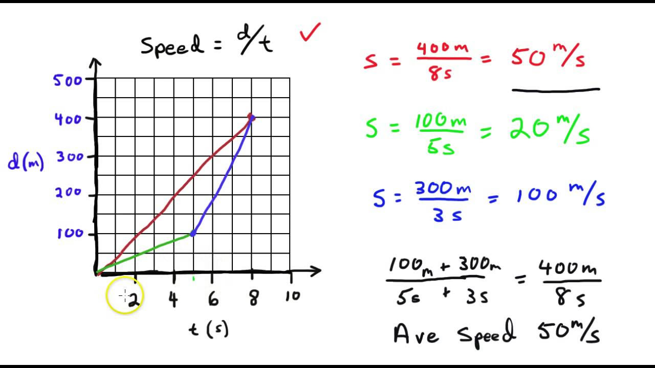
Image taken from the YouTube channel Takata Science , from the video titled Speed graphs – Average speed pt1 .
Imagine a Formula 1 race. The roar of the engines, the screech of tires, and the blur of cars speeding around the track. How do engineers and analysts make sense of this chaotic ballet of motion? One of their most powerful tools is the velocity-time graph.
Velocity-time graphs are not just abstract mathematical constructs. They are vital instruments for dissecting and understanding motion in countless real-world scenarios, from the design of high-speed trains to the analysis of a baseball player’s swing. This article will act as your comprehensive guide to demystifying these graphs.
The Power of Visualizing Motion
A velocity-time graph provides a visual representation of an object’s velocity over a specific period. But why is this visual representation so crucial?
Because it transforms complex data into an easily digestible format.
By plotting velocity against time, we gain immediate insights into how an object’s speed and direction change. This allows us to analyze acceleration, identify periods of constant velocity, and, most importantly, calculate average speed.
Defining Average Speed: Quantifying Motion
At its core, average speed is a fundamental concept in physics, representing the total distance traveled by an object divided by the total time taken.
It provides a single value that summarizes the overall rate of motion, regardless of whether the object’s speed was constant or varied during the journey.
Average speed, unlike velocity, is a scalar quantity, meaning it only considers the magnitude (numerical value) and not the direction.
Thesis Statement: Your Guide to Mastering Average Speed Calculations
This article aims to equip you with the knowledge and skills necessary to confidently calculate average speed from velocity-time graphs.
We will explore the underlying principles, delve into practical examples, and address common pitfalls, ensuring that you gain a solid understanding of this essential analytical technique. Prepare to unlock the secrets hidden within velocity-time graphs and gain a deeper appreciation for the world of motion.
Imagine a Formula 1 race. The roar of the engines, the screech of tires, and the blur of cars speeding around the track. How do engineers and analysts make sense of this chaotic ballet of motion? One of their most powerful tools is the velocity-time graph.
Velocity-time graphs are not just abstract mathematical constructs. They are vital instruments for dissecting and understanding motion in countless real-world scenarios, from the design of high-speed trains to the analysis of a baseball player’s swing. This article will act as your comprehensive guide to demystifying these graphs.
A velocity-time graph provides a visual representation of an object’s velocity over a specific period. But why is this visual representation so crucial?
Because it transforms complex data into an easily digestible format.
By plotting velocity against time, we gain immediate insights into how an object’s speed and direction change. This allows us to analyze acceleration, identify periods of constant velocity, and, most importantly, calculate average speed.
At its core, average speed is a fundamental concept in physics, representing the total distance traveled by an object divided by the total time taken.
It provides a single value that summarizes the overall rate of motion, regardless of whether the object’s speed was constant or varied during the journey.
Average speed, unlike velocity, is a scalar quantity, meaning it only considers the magnitude (numerical value) and not the direction.
Calculating average speed might seem straightforward on paper, but visualizing it on a velocity-time graph unlocks a deeper understanding. The graph serves as a dynamic map of motion, allowing us to "see" how speed changes over time, and how these changes contribute to the overall average. The next step involves understanding how to translate that visual information into concrete calculations.
Decoding Velocity-Time Graphs: A Visual Representation of Motion
Velocity-time graphs are more than just lines on a page. They are a visual language that describes the intricate dance of motion. Understanding this language is crucial for interpreting the story a graph tells about an object’s movement.
Axes: The Foundation of the Graph
The velocity-time graph is built on two fundamental axes:
-
The x-axis represents time, typically measured in seconds (s). It acts as the timeline of the motion.
-
The y-axis represents velocity, typically measured in meters per second (m/s). It indicates how fast and in what direction an object is moving at any given moment.
The values along the axes provide the raw data for interpreting the graph.
The Graph as a Storyteller of Motion
The magic of a velocity-time graph lies in its ability to visually represent changes in an object’s velocity over time.
A point on the graph reveals the instantaneous velocity at a specific time.
A continuous line shows how velocity evolves throughout the observed period.
A steep incline indicates a rapid increase in velocity.
A gentle slope represents a gradual change.
By tracing the line’s path, we can immediately grasp the dynamics of motion – acceleration, deceleration, or constant speed.
Slope: Unveiling Acceleration
The slope of the line on a velocity-time graph is not just an aesthetic feature; it’s a direct indicator of acceleration.
Acceleration, in this context, refers to the rate of change of velocity.
-
A positive slope signifies positive acceleration, meaning the object is speeding up in the positive direction.
-
A negative slope signifies negative acceleration, or deceleration, meaning the object is slowing down or accelerating in the negative direction.
-
A steep slope, whether positive or negative, indicates a large acceleration or deceleration.
-
A gentle slope shows a smaller acceleration or deceleration.
Steeper Slope vs. Gradual Slope
A steeper slope means a higher value of acceleration and shorter time duration for achieving the final velocity.
A gradual slope would mean that the object accelerates slowly over a long time duration.
Horizontal Lines: Constant Velocity
A horizontal line on a velocity-time graph is a special case. It represents constant velocity.
This means the object is moving at a steady speed, neither accelerating nor decelerating.
The velocity value remains the same throughout the time interval represented by the horizontal line. This is a state of equilibrium in terms of acceleration, where the net force acting on the object in the direction of motion is zero.
Negative Velocity: Direction Matters
The velocity-time graph is direction-sensitive. The y-axis extends into the negative region, representing motion in the opposite direction of the chosen positive direction.
If you define moving to the right as positive, then:
-
A positive velocity indicates movement to the right.
-
A negative velocity indicates movement to the left.
It is very important to account for the sign of velocity when calculating total distance traveled.
The fundamental nature of velocity-time graphs for understanding motion is now clear. The power to visualize changes in velocity over time opens the door to quantitative analysis, specifically the calculation of average speed.
Calculating Average Speed: Distance Over Time in Velocity-Time Graphs
At its core, average speed is a measure of how fast an object moves over a given duration. It’s a single value that summarizes the overall pace of motion, regardless of the complexities within the journey. Understanding how to extract this value from a velocity-time graph is the aim of this section.
Defining Average Speed: The Foundation of Motion Analysis
Let’s begin with the basics. Average speed is defined as the total distance traveled by an object divided by the total time taken.
Mathematically, it’s expressed as:
Average Speed = Total Distance / Total Time
This definition is critical, forming the bedrock upon which all our calculations will be based. Keep in mind that unlike velocity, which is a vector quantity possessing both magnitude and direction, average speed is a scalar quantity, focusing solely on magnitude.
The Area Under the Curve: Unlocking the Secrets of Displacement
The magic of velocity-time graphs lies in the geometric relationship between the graphed line and the axes. The area bounded between the velocity-time curve and the time axis holds a special significance: it represents the displacement of the object.
Displacement is the change in position of the object.
It’s important to remember that displacement can be positive or negative, depending on the direction of motion.
However, the area under the curve is not always equal to the total distance traveled. This distinction becomes important when the object changes direction during its motion, a subtlety we’ll address in a later section.
Calculating Total Distance from the Area
So how do we translate the area under the curve into the total distance traveled? This depends on whether the velocity is constant or changing.
-
Constant Velocity: If the velocity is constant, the velocity-time graph is a horizontal line. The area under the curve is simply a rectangle, and its area is calculated by:
Area = Velocity × Time.
This area directly corresponds to the distance traveled.
-
Varying Velocity: When the velocity changes, the graph becomes more complex. Here, we need to employ geometric principles. We may need to calculate the area of triangles, trapezoids, or even irregular shapes. If the shape is irregular, approximation techniques, such as dividing the area into smaller, more manageable shapes, are very useful.
It’s crucial to accurately calculate each area and sum them together to determine the total distance traveled. For more complex curves, integral calculus provides the most accurate method for calculating area, but for our purposes, we will focus on simpler geometric calculations.
Scenarios with Changing Direction
If the object moves in the opposite direction at all, this must be taken into account when calculating total distance. The area under the x-axis will be negative, and in order to find total distance, the absolute value of this area must be added to the area above the x-axis.
The Average Speed Formula: Putting It All Together
With the total distance and total time in hand, the final step is simple: Apply the average speed formula.
Average Speed = Total Distance / Total Time
This formula allows you to distill the information contained within a velocity-time graph into a single, meaningful value. This value represents the overall rate at which the object covered ground during the observed time interval.
By mastering this process, you unlock the ability to quantitatively analyze motion from a visual representation. This skill forms a powerful tool for understanding and predicting movement in diverse scenarios.
The magic of velocity-time graphs lies in the geometric relationship between the graphed line and the axes. The area bounded between the velocity-time curve and the time axis holds a special significance: it represents the displacement of the object.
Displacement is the change in position of the object.
It’s important to remember that displacement can be positive or negative, depending on the direction of motion. This contrasts with distance, which is always a positive scalar quantity.
Area Under the Curve: Unveiling Displacement and Distance
The area nestled beneath the curve of a velocity-time graph is far more than just a shaded region; it’s a treasure trove of information about an object’s motion. It allows us to determine both the displacement and the total distance traveled. However, extracting the correct information requires a careful understanding of the nuances between these two concepts and how they manifest on the graph.
Displacement: Area with Direction
The area under the velocity-time curve directly represents the displacement of the object.
Areas above the x-axis (where velocity is positive) contribute to positive displacement, indicating movement in the positive direction.
Conversely, areas below the x-axis (where velocity is negative) contribute to negative displacement, indicating movement in the opposite direction.
To calculate the total displacement, you must consider the sign of each area segment. Summing the positive areas and subtracting the negative areas will yield the net displacement.
For example, if an object moves 10 meters to the right (positive direction) and then 5 meters to the left (negative direction), the net displacement is +5 meters. This is reflected in the algebraic sum of the areas under the curve.
Total Distance: The Absolute Journey
While displacement tells us the net change in position, total distance represents the entire path traveled, regardless of direction.
Therefore, we cannot simply subtract areas below the x-axis when calculating total distance.
Instead, we must take the absolute value of each area segment.
This means that every area contributes a positive value to the total distance, reflecting the total ground covered during the motion.
Mathematically, the total distance is the sum of the absolute values of all area segments between the velocity-time curve and the time axis.
In our previous example, the object moved 10 meters to the right and 5 meters to the left. The total distance traveled is 10 meters + 5 meters = 15 meters.
This is calculated by summing the magnitudes of the areas under the curve, irrespective of their sign.
Calculating Areas: Geometric Approaches
To find the area under the curve, you’ll often need to divide the region into familiar geometric shapes: rectangles, triangles, and trapezoids. The standard formulas for area calculations then apply.
For more complex curves, integration (from calculus) provides a precise method to determine the area. However, for many introductory physics problems, geometric approximation is sufficient.
Carefully consider the units of velocity and time to ensure the resulting area (displacement/distance) is expressed in the correct units (e.g., meters).
Practical Examples: Applying Average Speed Calculations to Real-World Scenarios
Having explored the theoretical underpinnings of velocity-time graphs and their connection to displacement and distance, it’s time to put these concepts into action. By examining concrete, real-world scenarios, we can solidify our understanding of how to calculate average speed from these graphs and appreciate their practical applications.
Example 1: A Car Accelerating Uniformly
Imagine a car accelerating uniformly from rest. On a velocity-time graph, this scenario is represented by a straight line sloping upwards from the origin. Let’s say the car accelerates from 0 m/s to 20 m/s in 10 seconds.
Calculating the Total Distance
To determine the average speed during this acceleration phase, we first need to calculate the total distance traveled. This is represented by the area under the velocity-time graph, which in this case is a triangle.
The area of a triangle is (1/2) base height. Here, the base is the time interval (10 seconds), and the height is the final velocity (20 m/s).
Therefore, the area (and the distance traveled) is (1/2) 10 s 20 m/s = 100 meters.
Determining the Average Speed
Now that we know the total distance (100 meters) and the total time (10 seconds), we can calculate the average speed.
Average speed is defined as total distance divided by total time.
So, the average speed of the car during acceleration is 100 meters / 10 seconds = 10 m/s. This illustrates how a simple geometric calculation on a velocity-time graph reveals a key aspect of the car’s motion.
Example 2: A Runner with Varying Velocity
Consider a runner whose velocity changes throughout a race. Their motion is depicted on a velocity-time graph as a series of connected line segments, each representing a period of constant acceleration or deceleration.
Analyzing the Velocity-Time Graph
The velocity-time graph might show the runner accelerating at the start, maintaining a steady pace in the middle, and then slowing down towards the end of the race. Each of these phases is represented by a different segment on the graph.
Calculating Total Distance and Average Speed
To calculate the average speed over the entire race, we need to determine the total distance traveled and the total time taken. The total distance is found by calculating the area under the entire velocity-time curve.
This might involve dividing the area into simpler geometric shapes (triangles, rectangles, and trapezoids), calculating the area of each shape individually, and then summing them up.
Once the total distance is known, dividing it by the total time will give us the average speed of the runner over the entire race. This average speed provides a concise summary of the runner’s performance, even though their velocity varied throughout.
Example 3: Object Moving in Multiple Directions
Now, let’s examine a more complex scenario where an object moves in multiple directions. This is represented on a velocity-time graph by areas both above and below the x-axis.
Understanding Negative Velocity
Remember, areas above the x-axis represent movement in the positive direction, while areas below the x-axis represent movement in the negative direction. The key difference lies in calculating total distance versus displacement.
Calculating Total Distance
To find the total distance traveled, we must take the absolute value of each area segment. Add together areas above the x-axis, and the absolute value of areas below the x-axis.
This is because distance is a scalar quantity and always positive.
Calculating Displacement and Average Velocity
Displacement, on the other hand, is a vector quantity and considers direction. To find displacement, you’d sum areas above the x-axis and subtract the areas below the x-axis. Average velocity is Displacement / Time.
Calculating Average Speed
Once you have the total distance, divide it by the total time. This gives the average speed of the object, regardless of the changes in direction. For instance, imagine a remote-controlled car moving 5 meters forward then 2 meters in reverse in 7 seconds. The total distance is 7 meters but the average speed will be 1 m/s.
These examples demonstrate the power and versatility of velocity-time graphs in analyzing real-world motion. By understanding how to interpret these graphs and calculate the area under the curve, we can gain valuable insights into the movement of objects around us. The key is to remember the fundamental relationship between the graph, distance, displacement, and ultimately, average speed.
Having demonstrated the calculation of average speed through practical examples, a broader question emerges: how do these calculations fit within the larger framework of motion analysis?
Kinematics and Velocity-Time Graphs: A Symbiotic Relationship
The study of motion, known as kinematics, provides the foundational principles for understanding the movement of objects without considering the forces that cause that motion.
Velocity-time graphs are not merely visual aids; they are essential tools within the field of kinematics, offering a powerful means of representing and analyzing motion.
Kinematics: The Foundation of Motion Analysis
Kinematics deals with concepts such as displacement, velocity, acceleration, and time. It provides the vocabulary and the mathematical framework for describing how objects move.
Velocity-time graphs visually encapsulate these kinematic variables, presenting a comprehensive picture of an object’s motion over a specific time interval.
Consider a scenario where an object’s velocity is changing non-uniformly. Kinematic equations alone might not provide a straightforward solution.
However, a velocity-time graph allows us to visualize this changing velocity and, by determining the area under the curve, calculate the object’s displacement, even in complex scenarios.
Average Speed as a Key Kinematic Parameter
Average speed, as determined from velocity-time graphs, becomes a crucial parameter in kinematic analysis.
It provides a single value that summarizes the overall rate of motion during a given time interval.
This value can then be used in conjunction with other kinematic variables, such as acceleration and time, to make predictions about future motion or to analyze past motion.
For example, knowing the average speed of a car during a trip allows us to estimate the total distance traveled, even if the car’s speed varied throughout the journey.
Moreover, in situations where acceleration is constant, average speed can be directly related to initial and final velocities through kinematic equations, further highlighting its importance in problem-solving.
In essence, average speed, calculated from velocity-time graphs, bridges the gap between visual representation and quantitative analysis in kinematics, offering a powerful tool for understanding and predicting motion.
Having demonstrated the calculation of average speed through practical examples, a broader question emerges: how do these calculations fit within the larger framework of motion analysis?
Avoiding Pitfalls: Common Mistakes in Average Speed Calculations
Calculating average speed from velocity-time graphs might seem straightforward, but several common errors can lead to inaccurate results. Understanding these pitfalls and learning how to avoid them is crucial for accurate motion analysis. This section will highlight these potential mistakes and provide practical tips to ensure your calculations are precise.
Displacement vs. Distance: A Critical Distinction
One of the most frequent sources of error lies in confusing displacement and distance. Displacement is a vector quantity, representing the change in position of an object. It considers direction. Distance, on the other hand, is a scalar quantity, representing the total path length traveled by the object, irrespective of direction.
When calculating average speed, we are interested in the total distance traveled, not the displacement. This distinction becomes particularly important when the object changes direction.
The Impact of Direction Changes
Consider an object moving forward (positive velocity) and then backward (negative velocity). The area under the curve for the forward motion will be positive, while the area under the curve for the backward motion will be negative.
To find the displacement, you would add these areas algebraically (positive areas minus negative areas). However, to find the total distance, you must take the absolute value of each area and add them together. Failing to do so will result in an underestimation of the total distance and, consequently, an inaccurate average speed.
Remember: Average speed = (Total Distance Traveled) / (Total Time). Always calculate total distance by considering the absolute values of areas representing movement in different directions.
The Perils of Inaccurate Area Calculation
The area under the velocity-time curve is the cornerstone of distance and displacement calculation. However, errors in determining this area can significantly impact the accuracy of your average speed calculation.
Geometric Shapes and Their Precise Measurement
Often, the area under the curve can be divided into simple geometric shapes like rectangles, triangles, and trapezoids. Ensure you are using the correct formulas for calculating the area of each shape.
For example:
- Rectangle: Area = base × height
- Triangle: Area = 0.5 × base × height
- Trapezoid: Area = 0.5 × (base1 + base2) × height
Pay close attention to the units of measurement for the base and height, ensuring they are consistent (e.g., seconds for time and m/s for velocity). Double-check your calculations to avoid simple arithmetic errors.
Handling Complex Curves
When dealing with more complex curves that cannot be easily divided into standard geometric shapes, consider using approximation techniques. One common method is to divide the area into smaller rectangles or trapezoids and sum their areas.
The smaller the width of these individual shapes, the more accurate your approximation will be. In advanced scenarios, integral calculus can provide a precise calculation of the area under any curve defined by a mathematical function.
Ignoring Changes in Direction: A Recipe for Error
As previously emphasized, failing to account for changes in direction is a significant pitfall. It’s easy to overlook the sign of the velocity and treat all areas under the curve as positive, leading to an underestimation of the total distance traveled.
The Importance of the Velocity Sign
Whenever the velocity-time graph crosses the x-axis, it indicates a change in direction. The area above the x-axis represents motion in one direction (positive), while the area below the x-axis represents motion in the opposite direction (negative).
Before calculating the total distance, carefully examine the graph and identify any instances where the velocity changes sign. Treat the areas above and below the x-axis separately, taking the absolute value of each area before adding them together.
By diligently avoiding these common mistakes – confusing displacement with distance, incorrectly calculating area, and ignoring changes in direction – you can ensure accurate and reliable average speed calculations from velocity-time graphs.
Having demonstrated the calculation of average speed through practical examples, a broader question emerges: how do these calculations fit within the larger framework of motion analysis?
Beyond the Basics: Advanced Applications of Velocity-Time Graphs
While understanding the fundamentals of velocity-time graphs is essential, their true power lies in their ability to unlock insights into more complex scenarios. These graphs are not just tools for calculating average speed; they are windows into the intricate dance of motion, revealing patterns and allowing for predictions that extend far beyond simple uniform movement.
Analyzing Complex Motion Patterns
Velocity-time graphs shine when dissecting intricate motion such as oscillatory motion, exemplified by a swinging pendulum or a bouncing spring. Instead of a straight line or simple curve, these graphs exhibit repeating patterns.
The cyclical nature of oscillatory motion is immediately apparent, with the graph oscillating above and below the x-axis, showing alternating positive and negative velocities. The frequency and amplitude of these oscillations, directly extracted from the graph, provide valuable information about the system’s behavior.
Damped motion, where oscillations gradually decrease over time due to energy loss, presents a further layer of complexity. The velocity-time graph for damped motion will show oscillations with decreasing amplitude, visually representing the dissipation of energy.
Analyzing the rate at which the amplitude decays can provide insights into the damping forces acting on the system.
By carefully examining the shape and characteristics of these velocity-time graphs, we can gain a deeper understanding of the forces and energy transfers at play.
Predicting Future Motion
Beyond analyzing past and present motion, velocity-time graphs can be used to forecast future movement.
If we know the initial conditions (position and velocity) of an object and can model the forces acting upon it, we can extrapolate the velocity-time graph into the future.
This allows us to predict the object’s velocity and position at any given time. However, it’s crucial to acknowledge the limitations of such predictions. Real-world scenarios often involve factors that are difficult to model accurately, such as friction, air resistance, and unpredictable external forces.
Therefore, predictions based on velocity-time graphs are most reliable over short time intervals and under controlled conditions.
Connecting to Energy and Momentum
Velocity-time graphs provide a visual bridge to understanding fundamental physics concepts like energy and momentum.
Kinetic energy, the energy of motion, is directly related to velocity (KE = 1/2 mv²). By examining the velocity-time graph, we can infer changes in kinetic energy over time. A steeper slope indicates a greater change in velocity and, consequently, a greater change in kinetic energy.
Momentum, a measure of an object’s mass in motion (p = mv), is also directly linked to velocity.
The area under the curve, representing the change in position, is related to impulse, which is the change in momentum.
By analyzing the changes in velocity depicted in a velocity-time graph, we can gain insights into how energy is being transferred and how momentum is being conserved within a system. This holistic view strengthens our understanding of the underlying physical principles governing the motion.
FAQs: Unlocking Average Speed Secrets in Velocity-Time Graphs
Still have questions about velocity-time graphs and calculating average speed? Here are some common questions to help clarify the concepts.
What exactly does the area under a velocity-time graph represent?
The area under a velocity-time graph represents the displacement of the object. In simpler terms, it’s the total distance the object traveled in a specific direction. Calculating this area is crucial for finding the average speed in a velocity-time graph.
How is average speed different from instantaneous speed when looking at a velocity-time graph?
Instantaneous speed is the speed at a specific moment in time – you can read it directly off the velocity-time graph at that point. Average speed, on the other hand, considers the overall journey. It’s calculated by dividing the total distance traveled (area under the curve) by the total time.
Can the average speed in a velocity-time graph ever be negative?
No, average speed cannot be negative. Speed is the magnitude of velocity and is always a positive value or zero. If you are calculating velocity, you should take the direction into consideration.
What if the velocity-time graph has both positive and negative velocity values? How do I find the total distance for calculating average speed in this case?
You need to calculate the area above the x-axis (positive velocity) and the area below the x-axis (negative velocity) separately. Then, take the absolute value of each area and add them together. This gives you the total distance traveled, which you then divide by the total time to find the average speed in the velocity-time graph.
So, there you have it! Figuring out the average speed in velocity times graph doesn’t have to be a headache. Go practice, and you’ll be a pro in no time!
